# Johnson-Neyman intervals library(interactions)johnson_neyman(mod_interact, pred ="age", modx ="exercise")
JOHNSON-NEYMAN INTERVAL
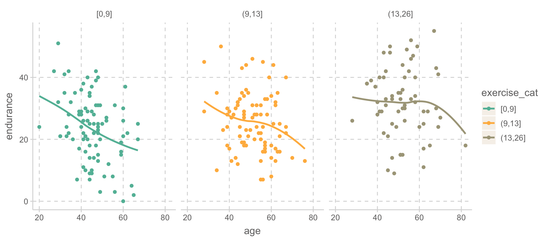
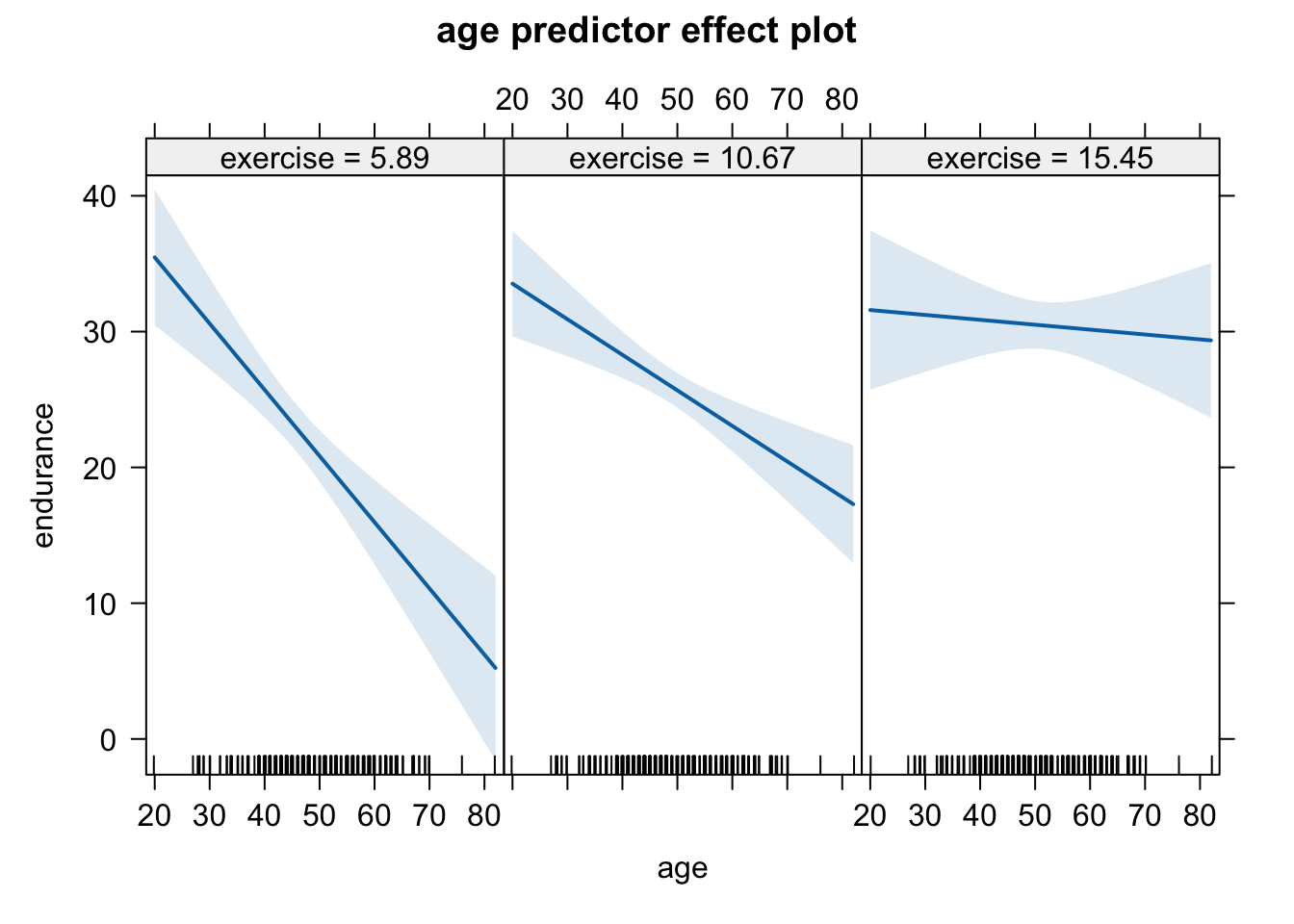
When exercise is OUTSIDE the interval [13.21, 24.37], the slope of age is p
< .05.
Note: The range of observed values of exercise is [0.00, 26.00]
Analysis of Variance Table

Model 1: endurance ~ age + exercise
Model 2: endurance ~ age * exercise
  Res.Df   RSS Df Sum of Sq     F    Pr(>F)
1    242 23810
2    241 22674  1    1136.5 12.08 0.0006042 ***
---
Signif. codes:  0 '***' 0.001 '**' 0.01 '*' 0.05 '.' 0.1 ' ' 1
Hayes의 PROCESS 매크로
Model 1
디폴트로 moderator의 16th, 50th, 84th 세 값에 대한 조건부 효과를 계산
moments=1: moderator의 mean, mean+sd, mean-sd 세 값에 대한 조건부 효과를 계산
wmodval=c(a, b, c)는 moderator 값이 a, b, c일 때의 조건부 효과를 계산
jn=1: Johnson-Neyman interval 계산
center=1: centering
process(data=acad2, y="endurance", x="age", w="exercise", model=1, center=1, jn=1)# ********************* PROCESS for R Version 4.3.1 ********************* # Written by Andrew F. Hayes, Ph.D. www.afhayes.com # Documentation available in Hayes (2022). www.guilford.com/p/hayes3 # *********************************************************************** # Model : 1 # Y : endurance# X : age # W : exercise # Sample size: 245# *********************************************************************** # Outcome Variable: endurance# Model Summary: # R R-sq MSE F df1 df2 p# 0.4540 0.2061 94.0821 20.8585 3.0000 241.0000 0.0000# Model: # coeff se t p LLCI ULCI# constant 25.8887 0.6466 40.0371 0.0000 24.6150 27.1625# age -0.2617 0.0641 -4.0848 0.0001 -0.3879 -0.1355# exercise 0.9727 0.1365 7.1244 0.0000 0.7038 1.2417# Int_1 0.0472 0.0136 3.4757 0.0006 0.0205 0.0740# Product terms key:# Int_1 : age x exercise # Test(s) of highest order unconditional interaction(s):# R2-chng F df1 df2 p# X*W 0.0398 12.0804 1.0000 241.0000 0.0006# ----------# Focal predictor: age (X)# Moderator: exercise (W)# Conditional effects of the focal predictor at values of the moderator(s):# exercise effect se t p LLCI ULCI# -4.6735 -0.4825 0.0911 -5.2935 0.0000 -0.6620 -0.3029# 0.3265 -0.2463 0.0641 -3.8403 0.0002 -0.3726 -0.1199# 4.3265 -0.0573 0.0861 -0.6656 0.5063 -0.2268 0.1123# Moderator value(s) defining Johnson-Neyman significance region(s):# Value % below % above# 2.5328 73.8776 26.1224# 13.6954 99.1837 0.8163# Conditional effect of focal predictor at values of the moderator:# exercise effect se t p LLCI ULCI# -10.6735 -0.7660 0.1598 -4.7931 0.0000 -1.0807 -0.4512# -9.3050 -0.7013 0.1430 -4.9057 0.0000 -0.9829 -0.4197# -7.9366 -0.6367 0.1266 -5.0288 0.0000 -0.8860 -0.3873# -6.5682 -0.5720 0.1110 -5.1552 0.0000 -0.7906 -0.3534# -5.1998 -0.5074 0.0964 -5.2647 0.0000 -0.6972 -0.3175# -3.8314 -0.4427 0.0834 -5.3087 0.0000 -0.6070 -0.2784# -2.4629 -0.3781 0.0729 -5.1863 0.0000 -0.5216 -0.2345# -1.0945 -0.3134 0.0661 -4.7437 0.0000 -0.4435 -0.1833# 0.2739 -0.2487 0.0641 -3.8809 0.0001 -0.3750 -0.1225# 1.6423 -0.1841 0.0674 -2.7312 0.0068 -0.3169 -0.0513# 2.5328 -0.1420 0.0721 -1.9699 0.0500 -0.2841 0.0000# 3.0107 -0.1194 0.0753 -1.5862 0.1140 -0.2678 0.0289# 4.3792 -0.0548 0.0865 -0.6332 0.5272 -0.2253 0.1157# 5.7476 0.0099 0.1000 0.0985 0.9216 -0.1871 0.2069# 7.1160 0.0745 0.1149 0.6484 0.5174 -0.1519 0.3009# 8.4844 0.1392 0.1308 1.0641 0.2883 -0.1184 0.3967# 9.8528 0.2038 0.1473 1.3839 0.1677 -0.0863 0.4939# 11.2213 0.2685 0.1642 1.6348 0.1034 -0.0550 0.5919# 12.5897 0.3331 0.1815 1.8354 0.0677 -0.0244 0.6906# 13.6954 0.3853 0.1956 1.9699 0.0500 0.0000 0.7707# 13.9581 0.3978 0.1990 1.9988 0.0468 0.0058 0.7898# 15.3265 0.4624 0.2167 2.1339 0.0339 0.0356 0.8893# ******************** ANALYSIS NOTES AND ERRORS ************************ # Level of confidence for all confidence intervals in output: 95# W values in conditional tables are the 16th, 50th, and 84th percentiles.# NOTE: The following variables were mean centered prior to analysis: # exercise age
Interaction의 패턴
Synergistic or enhancing interaction
상호작용 효과가 원래 효과들과 같은 방향으로 작용하는 경우
삶의 만족도(Y)가 직업 스트레스(X)와 부정적인 관계에 있고, 부부관계의 문제(Z)와도 부정적인 관계에 있는 경우
이 둘의 상호작용이 부정적이라면, 직업 스트레스와 부부관계의 문제가 동시에 증가하면 각각의 sum이 예측하는 것보다 더 낮은 삶의 만족도가 예측됨.
Buffering interaction
두 변수가 반대 방향으로 Y에 작용하고 있을 때, 한 변수가 다른 변수의 효과를 감소시키는 경우
즉, 한 변수의 impact가 다른 변수의 impact를 줄여주는 경우
건강보건에 대한 연구에서, 한 변수가 질병의 위험요인이고 다른 변수가 질병의 위험을 줄여주는 보호요인인 경우
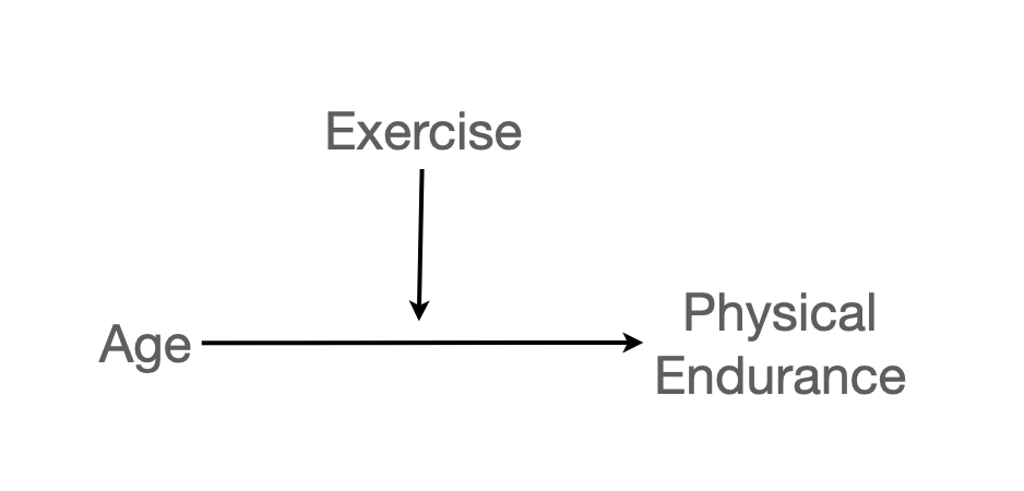
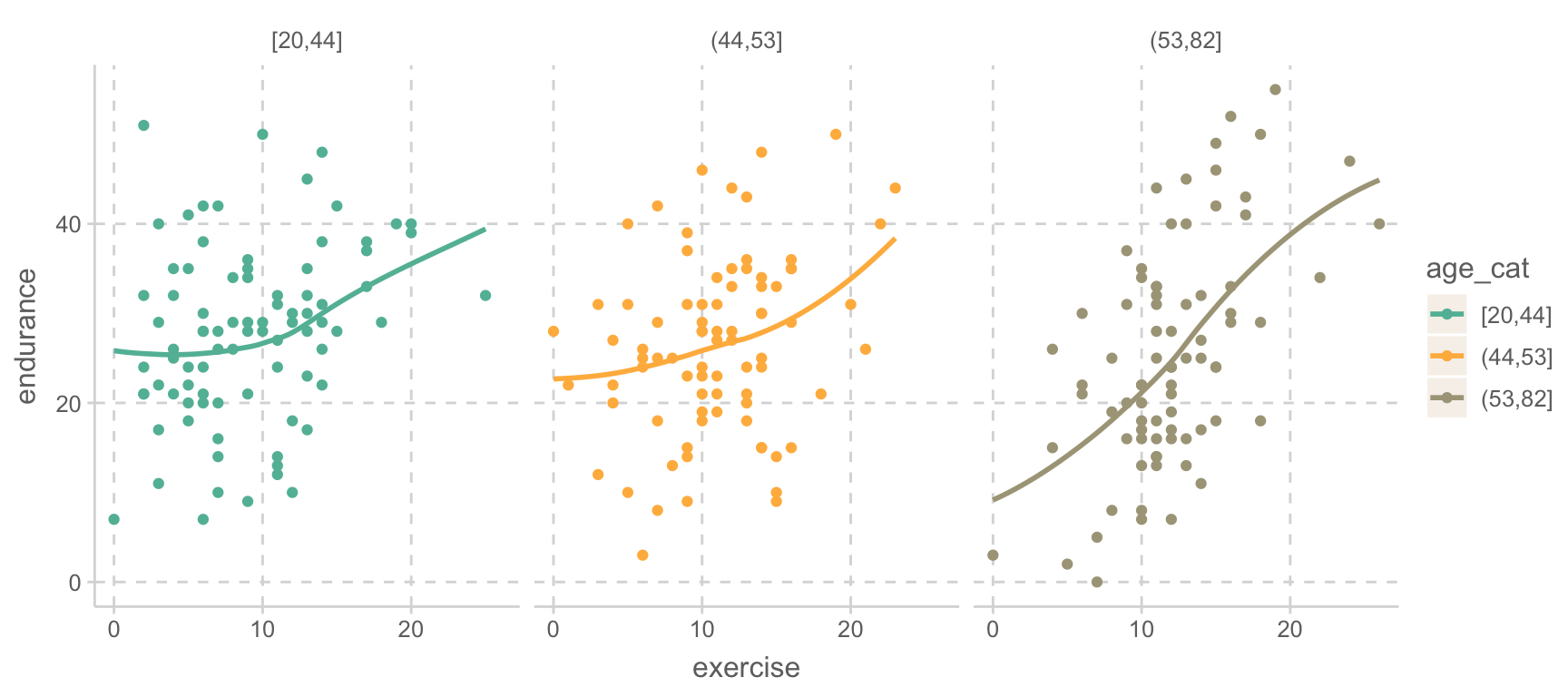
위의 예에서처럼, 나이(X)는 지구력 감소의 위험요인이고, 운동기간(Z)은 지구력 보호요인인 경우
Interference or antagonistic interactionin
두 변수가 같은 방향으로 Y에 작용하고 있을 때, 상호작용은 반대 방향으로 작용하는 경우
대학생의 학업성취도(Y)에 대하여, 학업동기(X)와 학업능력(Z)이 모두 학업성취도(Y)에 긍정적인 영향을 미치나 이 두 변수는 서로 보완적인 효과를 가지고 있음.
즉, 성취도에 대한 학업능력의 중요성은 높은 학업동기에 의해 낮아질 수 있음.
반대로, 학업동기에 대한 중요성은 높은 학업능력에 의해 낮아질 수 있음.
예제 2
Source: p.551, Statistical Methods for Psychology (8e) by Dave C. Howell
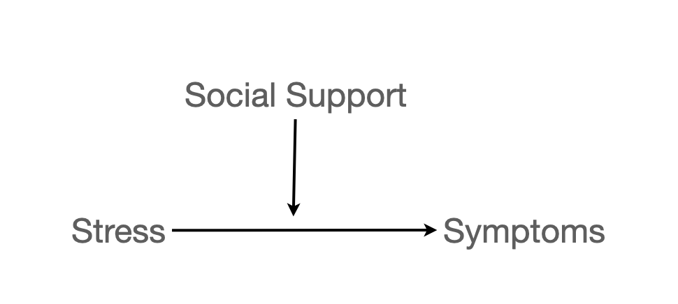
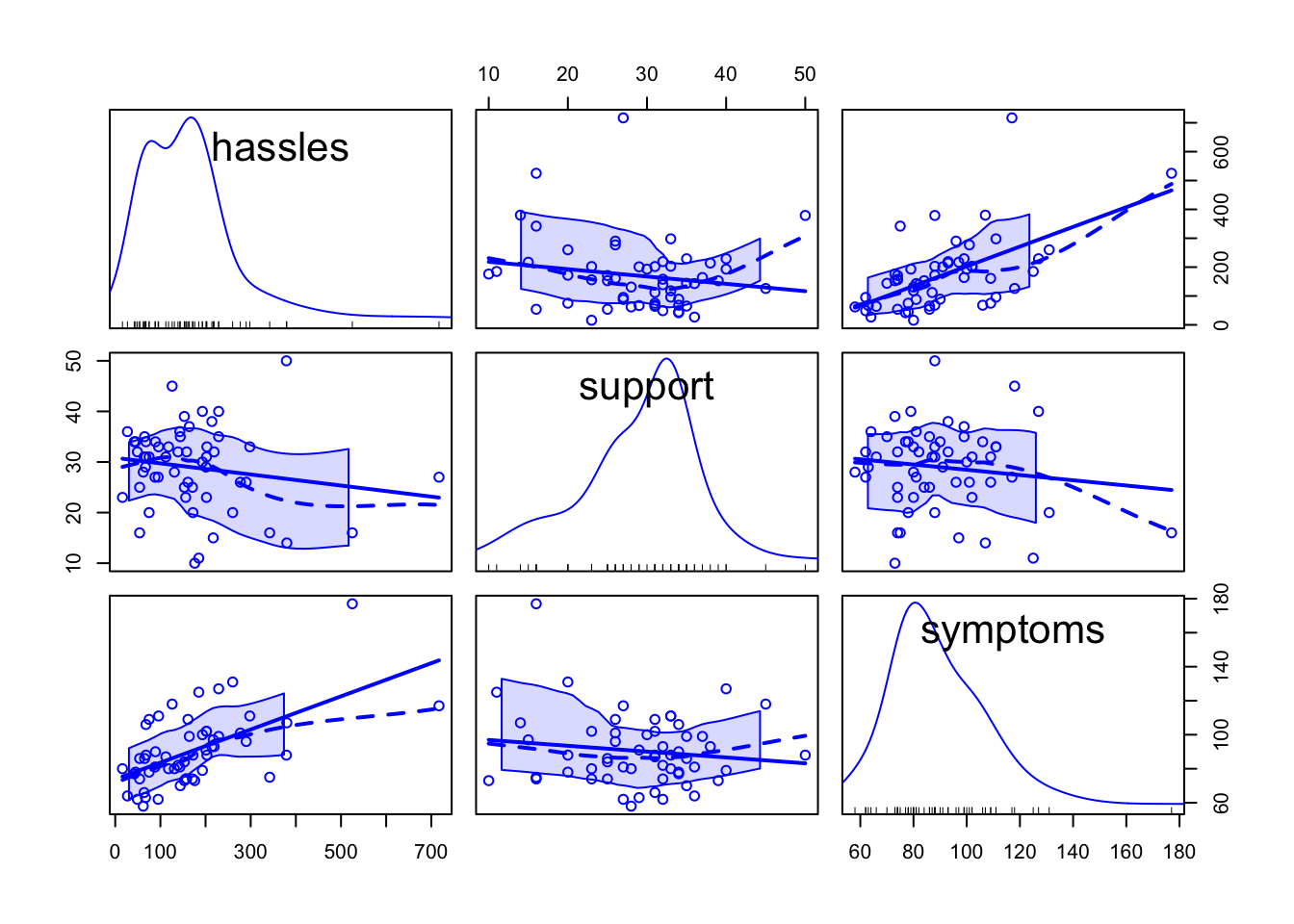
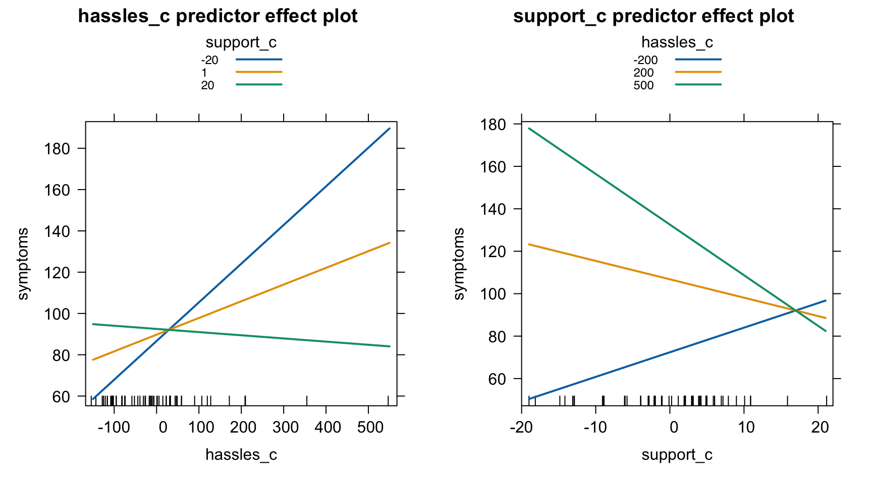
오리엔테이션에 참석한 대학 신입생을 대상으로, 스트레스 받은 일(hassles)이 많을 수록 여러 증상들(symptoms)을 더 경험하는데, 주위의 지지(support)가 많을 수록 그 증상들이 감소한다는 것을 알아보고자 설문 조사. (Wagner, Compas, and Howell (1988))
library(effects)# 임의의 3 levels 선택predictorEffects(mod, xlevels =3) |># 임의의 3 levels 선택plot(lines =list(multiline =TRUE)) # 3개의 선을 함께 그림
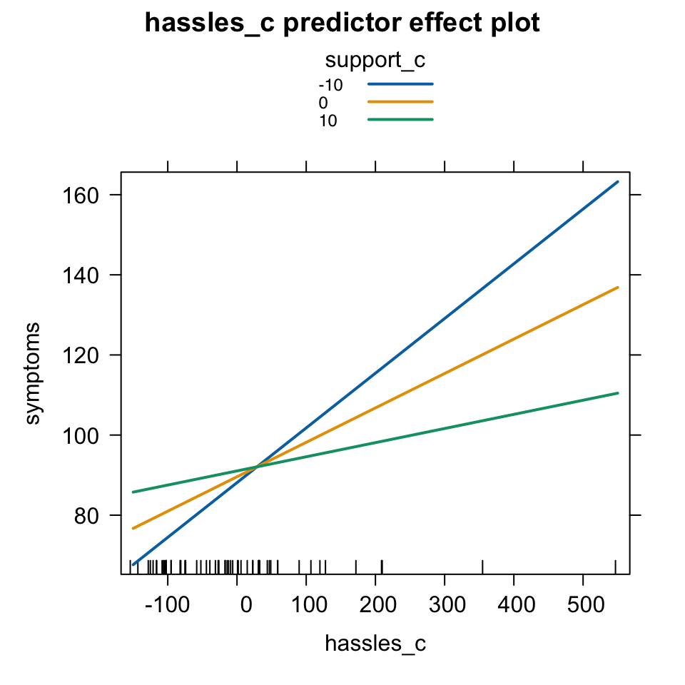
# 특정 3 levels 선택: -10(평균-10), 0(평균), 10(평균+10)predictorEffects(mod, ~ hassles_c, xlevels =list(support_c =c(-10, 0, 10))) |># 특정 3 levels 선택plot(lines =list(multiline =TRUE)) # 3개의 선을 함께 그림
# Johnson-Neyman intervals library(interactions)johnson_neyman(mod, pred ="hassles_c", modx ="support_c")
JOHNSON-NEYMAN INTERVAL

When support_c is OUTSIDE the interval [6.25, 297.50], the slope of
hassles_c is p < .05.

Note: The range of observed values of support_c is [-18.96, 21.04]
# A tibble: 3 × 11
   wage  educ race  sex   hispanic south married exper union   age sector
  <dbl> <int> <fct> <fct> <fct>    <fct> <fct>   <int> <fct> <int> <fct>
1   9      10 W     M     NH       NS    Married    27 Not      43 const
2   5.5    12 W     M     NH       NS    Married    20 Not      38 sales
3   3.8    12 W     F     NH       NS    Single      4 Not      22 sales
편의상 management 섹터에서만 보면,
cps <- cps |>filter(sector =="manag") |>filter(wage <30& age <60) |>slice(-51)
cps |>ggplot(aes(x = age, y = wage, color = sex)) +geom_point() +geom_smooth(se=F)
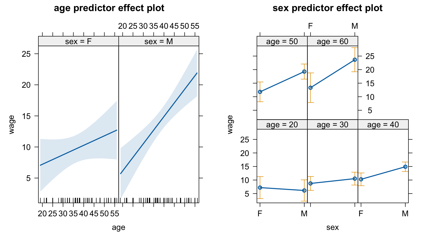
\(\hat{wage} = b_0 + b_1\cdot age + b_2\cdot sexM + b_3\cdot age \cdot sexM\)
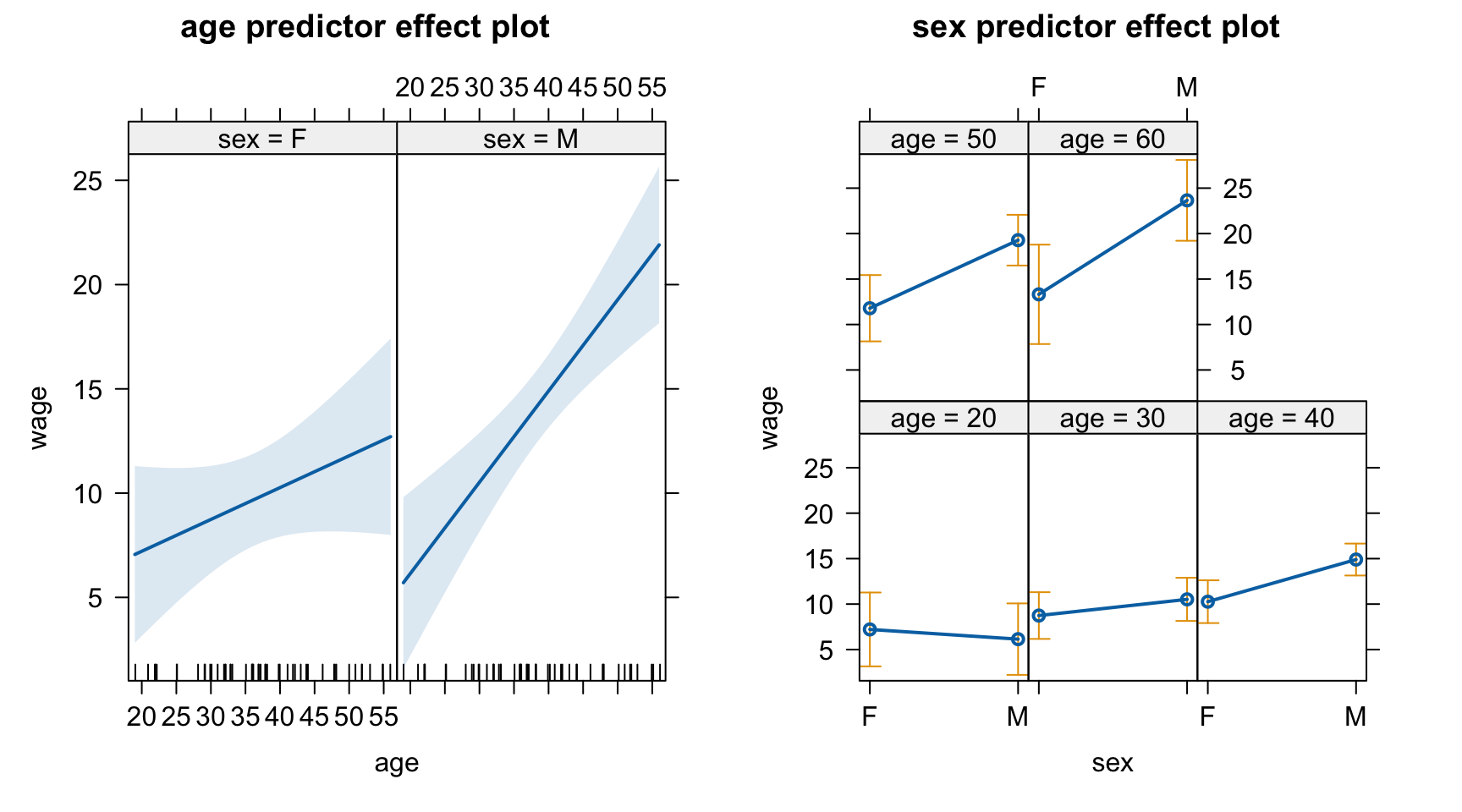
mod <-lm(wage ~ age * sex, data = cps)S(mod)
Call: lm(formula = wage ~ age * sex, data = cps)

Coefficients:
            Estimate Std. Error t value Pr(>|t|)
(Intercept)   4.1600     3.9354   1.057   0.2960
age           0.1526     0.1044   1.463   0.1504
sexM         -6.7728     5.4323  -1.247   0.2188
age:sexM      0.2852     0.1409   2.025   0.0487 *
---
Signif. codes:  0 '***' 0.001 '**' 0.01 '*' 0.05 '.' 0.1 ' ' 1

Residual standard deviation: 4.795 on 46 degrees of freedom
Multiple R-squared: 0.4266
F-statistic: 11.41 on 3 and 46 DF,  p-value: 1.028e-05
   AIC    BIC
304.47 314.03
predictorEffects(mod) |>plot()
상호작용항의 추가 설명력: \(\Delta R^2\) 계산
mod <-lm(wage ~ age * sex, data = cps)mod_reduced <-lm(wage ~ age + sex, data = cps)r2_full <-summary(mod)$r.squaredr2_reduced <-summary(mod_reduced)$r.squaredsprintf("R2 diff: %.3f", r2_full - r2_reduced)
[1] "R2 diff: 0.051"
anova(mod_reduced, mod)
Analysis of Variance Table

Model 1: wage ~ age + sex
Model 2: wage ~ age * sex
  Res.Df    RSS Df Sum of Sq      F  Pr(>F)
1     47 1151.7
2     46 1057.5  1     94.23 4.0991 0.04874 *
---
Signif. codes:  0 '***' 0.001 '**' 0.01 '*' 0.05 '.' 0.1 ' ' 1
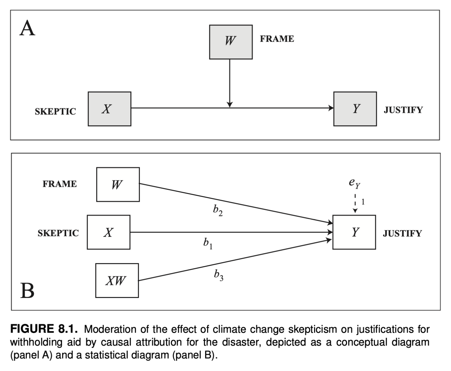
예제 2: 기후 변화 회의론이 원조 보류의 정당성에 미치는 영향
p. 285, Introduction to Mediation, Moderation, and Conditional Process Analysis (3e) by Andrew F. Hayes
연구 설명
저는 7장에서 소개한 조절 분석 방법을 재난의 원인을 기후 변화로 돌리는 것과 원인을 특정하지 않는 것이 기후 변화의 현실에 대한 사람들의 믿음에 따라 피해자에 대한 지원을 보류하는 사람들의 정당성에 차별적으로 영향을 미치는지 조사한 연구 데이터를 사용하여 설명했습니다. 이 예에서 초점 선행 변수는 가뭄의 원인에 대한 프레임을 코딩하는 이분법적 변수였고, 조절 변수는 기후 변화의 현실에 대한 회의론의 연속선상에 각 사람을 위치시키는 측정된 개인적 차이였습니다. 분석 결과, 기후 변화에 대해 회의적인 사람들은 원인을 특정하지 않은 경우보다 기후 변화로 인한 재난일 때 원조 보류에 대한 더 강력한 정당성을 보고했습니다. 기후 변화에 대한 회의적 시각이 상대적으로 낮은 사람들 사이에서는 이러한 효과가 관찰되지 않았습니다. 하지만 재난의 원인을 어떻게 규정하느냐가 아니라 기후변화 회의론이 재난 피해자에 대한 원조 의지에 미치는 영향에 실질적으로 초점을 맞춘다면 어떨까요? 이 질문은 간단한 회귀 분석으로 쉽게 답할 수 있습니다. 기후 변화 회의론(X)으로부터 원조 보류의 정당성(Y)을 추정하는 가장 적합한 OLS 회귀 모델은 Yˆ = 2.186+0.201X입니다. 따라서 기후 변화에 대한 회의론이 1단위 차이가 나는 두 사람은 기근 피해자에 대한 원조 보류의 정당성 강도에서 0.201단위 차이가 나는 것으로 추정됩니다. 이 관계는 통계적으로 유의미합니다. 그러나 이 분석은 이 연구 참여자의 절반은 가뭄과 그로 인한 기근이 기후 변화로 인한 것이라고 들었지만 다른 사람들은 그 원인에 대한 정보가 전혀 제공되지 않았다는 점을 완전히 무시하고 있습니다. 이 연구의 저자에 따르면, 기후 변화로 인한 것으로 표시된 사건은 기후 변화 회의론자들이 기후 변화의 현실에 대해 덜 회의적인 사람들에 비해 피해자를 돕는 것의 가치에 대해 특히 의심하게 만들 수 있다고 합니다. 즉, 기후 변화에 대한 귀인이 동기가 부여된 방어적 태도를 유발할 수 있으며, 기후 변화의 현실에 대한 태도는 그러한 귀인이 없을 때와 비교하여 도움에 대한 태도를 더 잘 예측할 수 있습니다. 다시 말해, 이러한 귀인은 사람들이 아무런 원인이 제공되지 않았을 때보다 자신의 태도와 더 일치하는 방식으로 피해자의 요구에 응답하도록 유도할 수 있습니다. 이러한 추론에 따르면 기후변화가 가뭄의 원인이라고 들었을 때와 원인에 대한 정보가 제공되지 않았을 때 기후변화 회의론과 원조 보류의 정당성 사이의 관계가 다를 것으로 예상할 수 있습니다. 기후변화 회의론 X와 재난 프레임 W(기후변화 조건은 1, 자연적 원인 조건은 0으로 설정)라고 부르면 7장에서와 마찬가지로 간단한 조정 모델을 추정할 수 있는데, 이 모델에서 X가 Y에 미치는 영향은 다음과 같다. 이러한 과정은 그림 8.1, 패널 A에 개념적으로 도식화되어 있으며 그림 8.1, 패널 B의 통계 다이어그램에서와 같이 X, W 및 XW를 선행 변수로 하는 통계 모형으로 변환됩니다.
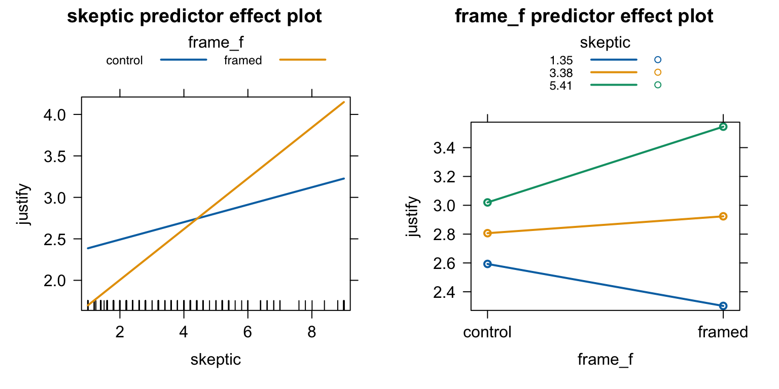
m <-mean(disaster$skeptic, na.rm =TRUE) |>round(2)sd <-sd(disaster$skeptic, na.rm =TRUE) |>round(2)predictorEffects(mod, xlevels =list(skeptic =c(m-sd, m, m+sd))) |>plot(lines =list(multiline =TRUE)) # 3개의 선을 함께 그림
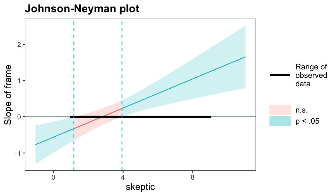
# johnson_neyman() 함수의 경우 카테고리 변수를 factor가 아닌 숫자로 입력해야 함mod2 <-lm(justify ~ skeptic * frame, data = disaster) # frame: 0, 1johnson_neyman(mod2, pred ="frame", modx ="skeptic")
JOHNSON-NEYMAN INTERVAL

When skeptic is OUTSIDE the interval [1.17, 3.93], the slope of frame is p
< .05.

Note: The range of observed values of skeptic is [1.00, 9.00]
상호작용항의 추가 설명력: \(\Delta R^2\) 계산
mod <-lm(justify ~ skeptic * frame_f, data = disaster)mod_reduced <-lm(justify ~ skeptic + frame_f, data = disaster)r2_full <-summary(mod)$r.squaredr2_reduced <-summary(mod_reduced)$r.squaredsprintf("R2 diff: %.3f", r2_full - r2_reduced)
# A tibble: 6 × 5
     ya    yb    yc lesion  drug
  <dbl> <dbl> <dbl> <chr>   <chr>
1  5.93 13.9   7.93 SURGERY ACTIVE
2  6.61 14.6   8.61 SURGERY ACTIVE
3  7.26 11.3   9.26 SHAM    PLACEBO
4  8.81  8.81 10.8  SURGERY PLACEBO
5  5.78 13.8   7.78 SURGERY ACTIVE
6 10.2  10.2  12.2  SURGERY PLACEBO
# A tibble: 5 × 11
   wage  educ race  sex   hispanic south married exper union   age sector
  <dbl> <int> <fct> <fct> <fct>    <fct> <fct>   <int> <fct> <int> <fct>
1   9      10 W     M     NH       NS    Married    27 Not      43 const
2   5.5    12 W     M     NH       NS    Married    20 Not      38 sales
3   3.8    12 W     F     NH       NS    Single      4 Not      22 sales
4  10.5    12 W     F     NH       NS    Married    29 Not      47 clerical
5  15      12 W     M     NH       NS    Married    40 Union    58 const
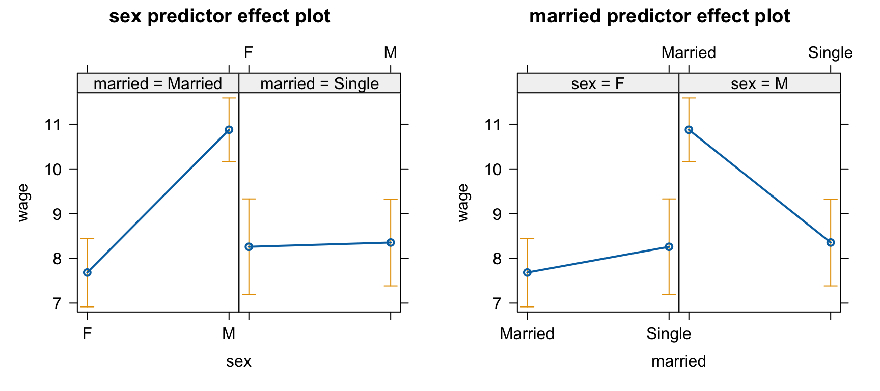
mod <-lm(wage ~ sex * married, data = cps)S(mod)
Call: lm(formula = wage ~ sex * married, data = cps)

Coefficients:
                   Estimate Std. Error t value Pr(>|t|)
(Intercept)          7.6838     0.3898  19.711  < 2e-16 ***
sexM                 3.1923     0.5319   6.002 3.62e-09 ***
marriedSingle        0.5759     0.6697   0.860  0.39026
sexM:marriedSingle  -3.0972     0.9073  -3.414  0.00069 ***
---
Signif. codes:  0 '***' 0.001 '**' 0.01 '*' 0.05 '.' 0.1 ' ' 1

Residual standard deviation: 4.962 on 530 degrees of freedom
Multiple R-squared: 0.07314
F-statistic: 13.94 on 3 and 530 DF,  p-value: 9.234e-09
    AIC     BIC
3232.05 3253.45
predictorEffects(mod) |>plot()
관찰연구의 경우 confounding이 될만한 통제 변수를 충분히 고려해야 하고, 나이가 성별과 결혼 여부와 상관관계가 있으므로 통제 변수로 포함.
cps |>select(age, sex, married) |>lowerCor()
         age   sex*  mrrd*
age       1.00
sex*     -0.08  1.00
married* -0.28  0.01  1.00
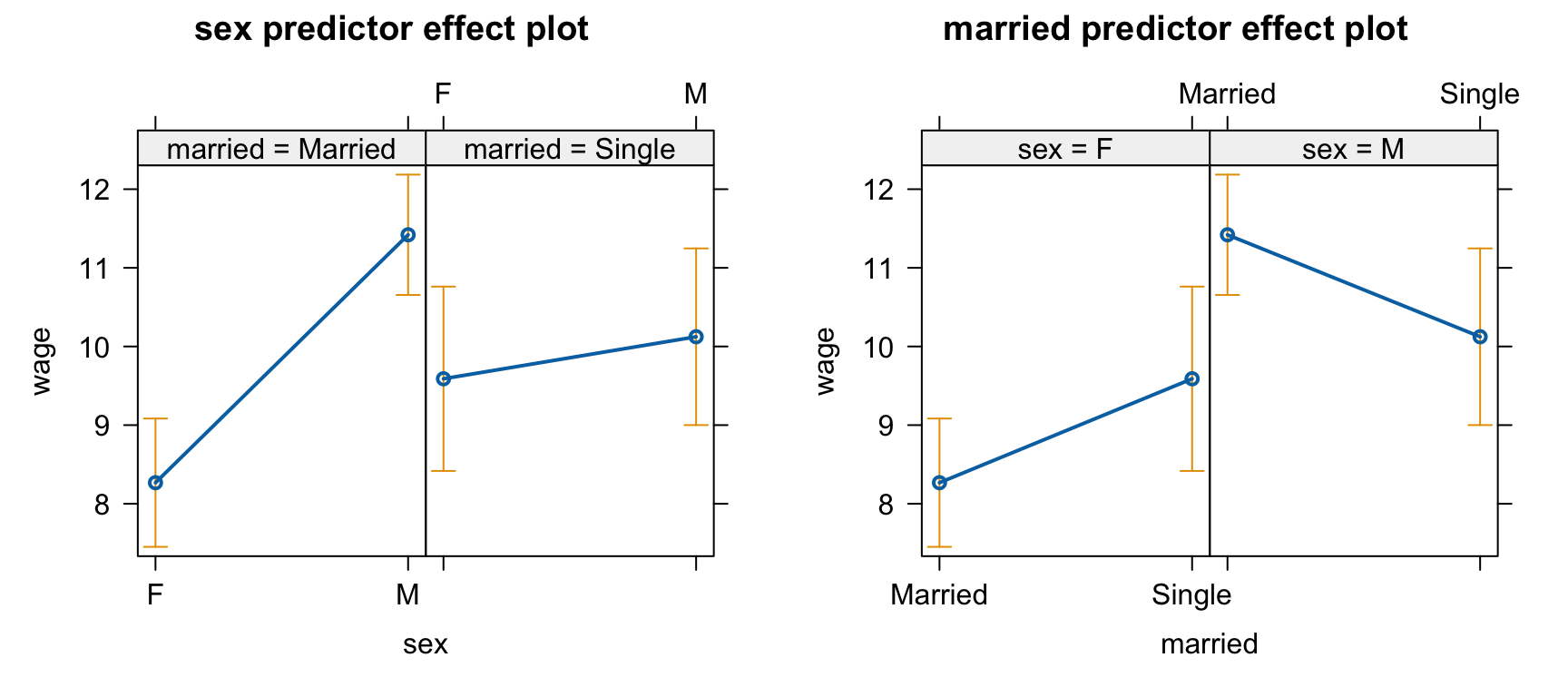
# age와 wage의 관계는 비선형적: spline regression (piecewise polynomial) fit을 고려할 필요있음mod2 <-lm(wage ~ sex * married + age +I(age^2), data = cps) predictorEffects(mod2, ~ sex + married) |>plot()
S(mod2)
Call: lm(formula = wage ~ sex * married + age + I(age^2), data = cps)

Coefficients:
                    Estimate Std. Error t value Pr(>|t|)
(Intercept)        -5.147951   2.391631  -2.152  0.03181 *
sexM                3.152425   0.516297   6.106 1.98e-09 ***
marriedSingle       1.321511   0.662608   1.994  0.04662 *
age                 0.608443   0.121565   5.005 7.62e-07 ***
I(age^2)           -0.006630   0.001483  -4.470 9.60e-06 ***
sexM:marriedSingle -2.617902   0.887868  -2.949  0.00333 **
---
Signif. codes:  0 '***' 0.001 '**' 0.01 '*' 0.05 '.' 0.1 ' ' 1

Residual standard deviation: 4.816 on 528 degrees of freedom
Multiple R-squared: 0.1301
F-statistic:  15.8 on 5 and 528 DF,  p-value: 1.649e-14
    AIC     BIC
3202.17 3232.13
결혼 유무에 따른 임금의 차이는 여성의 경우 미혼이 $1.32(p = 0.047) 높음.
남성의 경우는 아래와 같이 factor level을 변경해서 보면, 남성인 경우 미혼이 $1.29(p = 0.041) 낮음.
mod2_m <-lm(wage ~fct_relevel(sex, "M") * married + age +I(age^2), data = cps)S(mod2_m)
Call: lm(formula = wage ~ fct_relevel(sex, "M") * married + age + I(age^2),
         data = cps)

Coefficients:
                                      Estimate Std. Error t value Pr(>|t|)
(Intercept)                          -1.995525   2.393324  -0.834  0.40478
fct_relevel(sex, "M")F               -3.152425   0.516297  -6.106 1.98e-09 ***
marriedSingle                        -1.296391   0.632255  -2.050  0.04082 *
age                                   0.608443   0.121565   5.005 7.62e-07 ***
I(age^2)                             -0.006630   0.001483  -4.470 9.60e-06 ***
fct_relevel(sex, "M")F:marriedSingle  2.617902   0.887868   2.949  0.00333 **
---
Signif. codes:  0 '***' 0.001 '**' 0.01 '*' 0.05 '.' 0.1 ' ' 1

Residual standard deviation: 4.816 on 528 degrees of freedom
Multiple R-squared: 0.1301
F-statistic:  15.8 on 5 and 528 DF,  p-value: 1.649e-14
    AIC     BIC
3202.17 3232.13
Important
특히, 카테고리 변수와의 상호작용을 테스트할 때, 유닉크한 카테고리들의 조합에 해당하는 표본의 수가 급격히 줄기 때문에 표본의 수가 충분히 많아야 함.
예를 들어, 위의 경우 4가지 조합(싱글 남자, 싱글 여자, 기혼 남자, 기혼 여자)에 대한 표본의 수가 충분히 많아야 함.
Moderated Mediation
p. 424, Introduction to Mediation, Moderation, and Conditional Process Analysis (3e) by Andrew F. Hayes
연구 설명
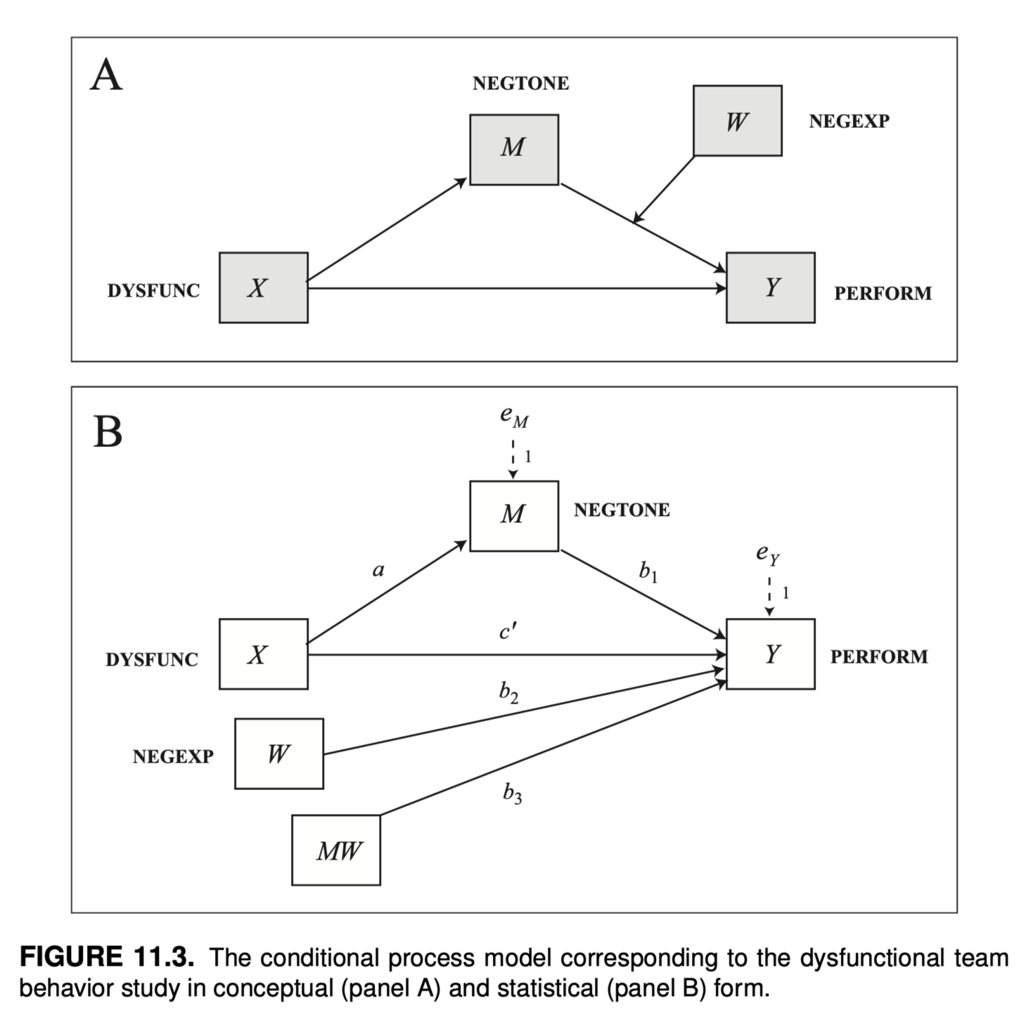
11.3 예시: 업무 팀에게 자신의 감정 숨기기 수년에 걸쳐 대중음악은 우리의 직관을 강화해왔고, 친한 친구들이 제공한 조언이나 친한 친구들이 제공하고 토크쇼 심리학자들은 감정을 억누르고 다른 사람의 눈에 띄지 않도록 숨겨서는 좋은 결과를 얻을 수 없다고 강조합니다. 당대의 아티스트들은 “자신을 표현하라”(마돈나)고, “침묵의 강령”(빌리 조엘)에 따라 살면 결코 과거를 잊지 못할 것이며 “절대 말하지 않을 것들”(에이브릴 라빈)의 목록이 길수록 인생에서 원하는 것을 얻을 가능성이 줄어든다는 것을 조심하라고 말합니다. 따라서 다른 사람이 “나랑 얘기 좀 하자”(아니타 베이커)는 요청을 할 때는 경계심을 풀고 마음속에 있는 이야기를 “소통”(B-52)하는 것이 중요합니다. 하지만 적어도 일부 업무 관련 상황에서는 반드시 그렇지는 않다고 M. S. Cole 외(2008)의 팀워크에 관한 연구에 따르면 말합니다. 이 연구자들에 따르면, 때로는 함께 일하는 다른 사람들이 자신을 괴롭히는 행동이나 말에 대해 자신의 감정을 숨기는 것이 더 나을 수 있으며, 그러한 감정이 팀의 관심의 초점이 되어 팀이 적시에 효율적인 방식으로 작업을 수행하는 데 방해가 되지 않도록 하는 것이 더 나을 수 있습니다. 이 연구는 조건부 프로세스 모델의 추정과 해석의 메커니즘을 설명하는 첫 번째 사례의 데이터를 TEAMS라는 데이터 파일로 제공하며, www.afhayes.com 에서 확인할 수 있습니다. 이 연구는 자동차 부품 제조 회사에 고용된 60개의 작업 팀을 대상으로 진행되었으며, 회사 직원 200여 명을 대상으로 작업 팀에 대한 일련의 질문과 팀 감독자에 대한 다양한 인식에 대한 설문조사에 대한 응답을 기반으로 합니다. 이 연구의 일부 변수는 그룹 수준에서 측정된 것으로 같은 팀원들이 말한 내용을 종합하여 도출한 것입니다. 다행히 팀원들이 팀에 대한 질문에 응답하는 방식이 매우 유사하여 이러한 종류의 집계를 정당화할 수 있었습니다. 다른 변수는 순전히 팀 상사의 보고를 기반으로 합니다.
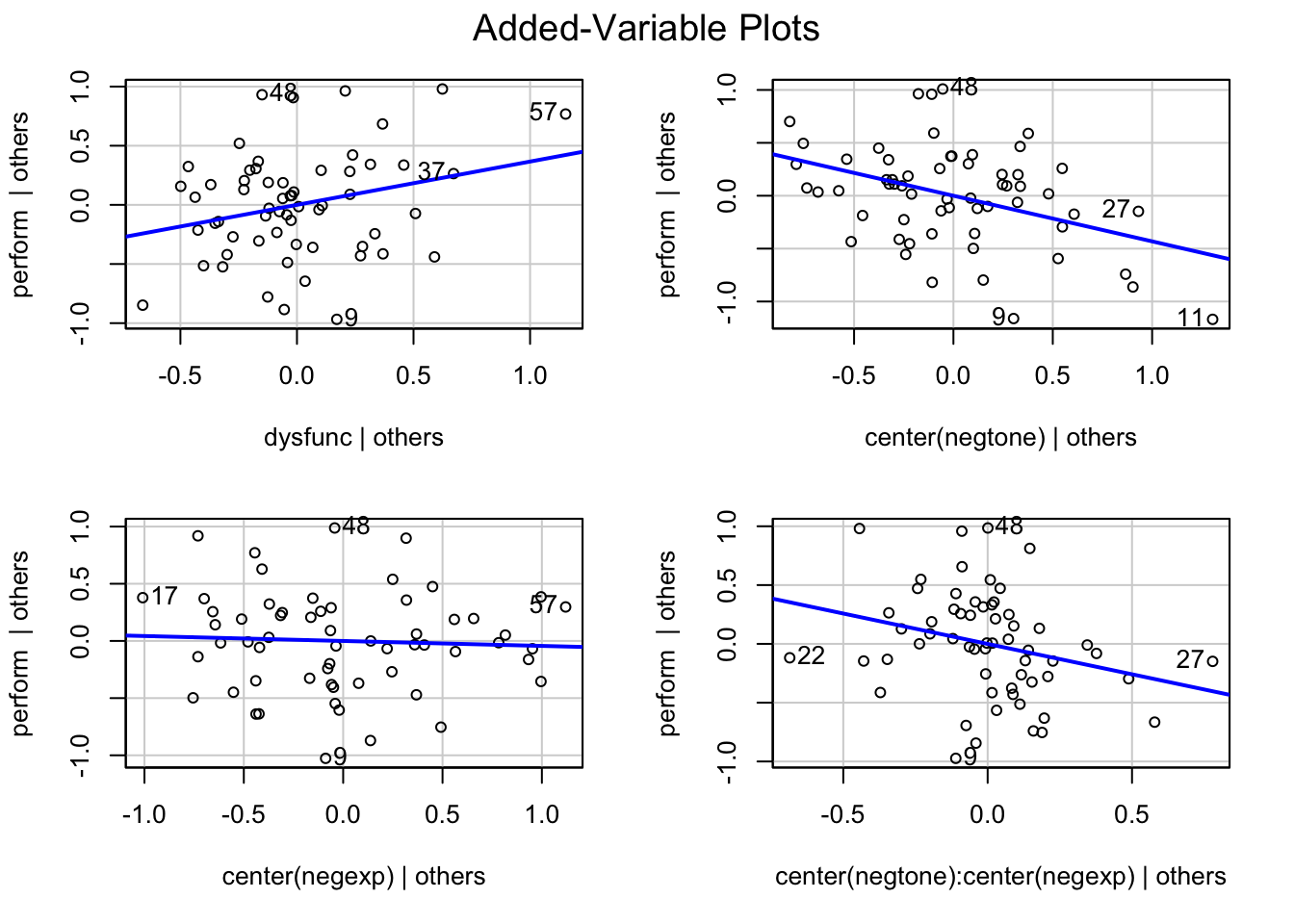
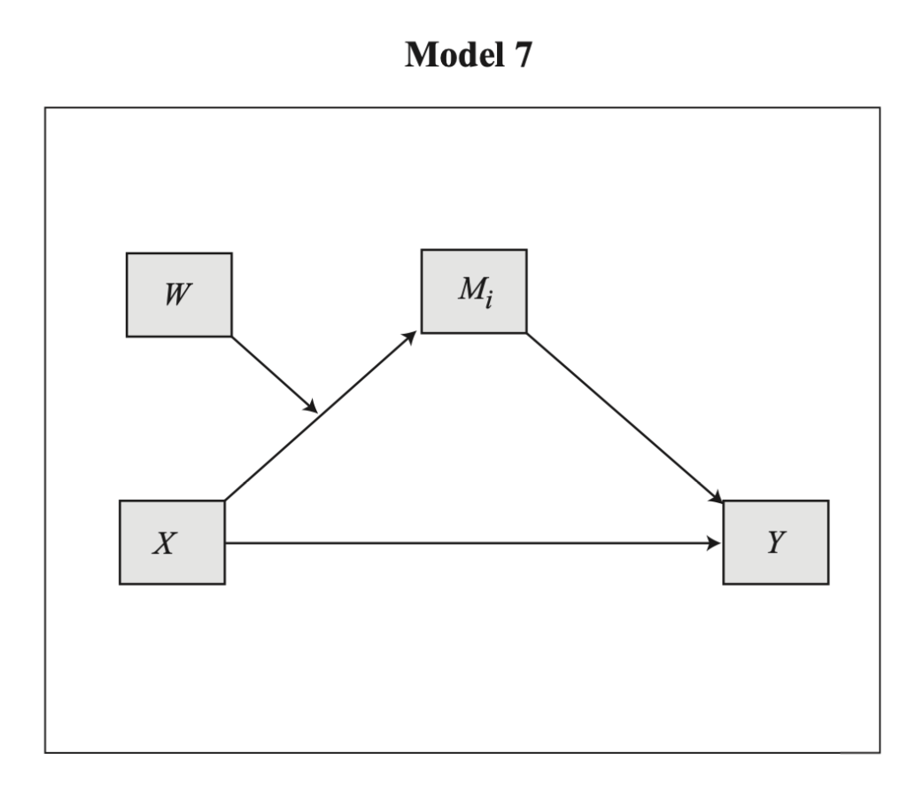
이 분석과 관련된 네 가지 변수를 측정했습니다. 팀원들이 다른 팀원들의 업무를 약화시키거나 변화와 혁신을 방해하는 행동을 얼마나 자주 했는지 등 팀원들의 역기능적 행동에 대한 일련의 질문(데이터 파일에서 DYSFUNC, 점수가 높을수록 팀 내 역기능적 행동이 많음을 나타냄)을 던져 팀원들의 역기능적 행동을 측정했습니다. 또한 팀원들에게 직장에서 ‘화가 났다’, ‘역겨웠다’ 등을 얼마나 자주 느끼는지 물어봄으로써 그룹의 부정적인 정서적 분위기를 측정했습니다(NEGTONE, 점수가 높을수록 업무 환경의 부정적인 정서적 분위기를 더 많이 반영함). 팀 상사에게는 팀이 얼마나 효율적이고 적시에 일을 처리하는지, 팀이 생산 목표를 달성하는지 등 전반적인 팀 성과에 대한 평가를 제공하도록 요청했습니다(데이터의 성과, 점수가 높을수록 성과가 좋음을 반영하는 척도). 또한 슈퍼바이저는 팀원들이 자신의 감정에 대해 보내는 비언어적 신호를 얼마나 쉽게 읽을 수 있는지를 측정하는 일련의 질문, 즉 비언어적 부정적 표현력(데이터 파일의 NEGEXP, 점수가 높을수록 팀원들이 부정적인 감정 상태를 비언어적으로 더 잘 표현한다는 의미)에 응답했습니다. 이 연구의 목표는 업무 팀원의 역기능적 행동이 업무 팀의 성과에 부정적인 영향을 미칠 수 있는 메커니즘을 조사하는 것이었습니다. 연구진은 역기능적 행동(X)으로 인해 상사와 다른 직원들이 직면하고 관리하려고 하는 부정적인 감정(M)으로 가득 찬 업무 환경이 조성되면 업무에 집중하지 못하고 업무 수행에 방해가 된다는 중재 모델을 제안했습니다(Y). 그러나 이 모델에 따르면 팀원들이 부정적인 감정(W)을 조절할 수 있게 되면, 즉 자신의 감정을 다른 사람에게 숨길 수 있게 되면 업무 환경의 부정적인 분위기와 다른 사람의 감정을 관리하는 데 집중할 필요 없이 당면한 업무에 집중할 수 있게 됩니다. 즉, 이 모델에서는 업무 환경의 부정적인 정서적 어조가 팀 성과에 미치는 영향은 팀원이 자신의 감정을 숨기는 능력에 따라 달라지며, 부정적 감정을 숨기지 않고 표현하는 팀에서 부정적인 정서적 어조가 성과에 미치는 부정적 영향이 더 강하다고 가정합니다.
mod_x <-lm(center(negtone) ~ dysfunc, data = teams)S(mod_x, brief = T)
Coefficients:
            Estimate Std. Error t value Pr(>|t|)
(Intercept) -0.02148    0.06176  -0.348 0.729182
dysfunc      0.61975    0.16683   3.715 0.000459 ***
---
Signif. codes:  0 '***' 0.001 '**' 0.01 '*' 0.05 '.' 0.1 ' ' 1

Residual standard deviation: 0.4763 on 58 degrees of freedom
Multiple R-squared: 0.1922
F-statistic:  13.8 on 1 and 58 DF,  p-value: 0.000459
  AIC   BIC
85.23 91.51
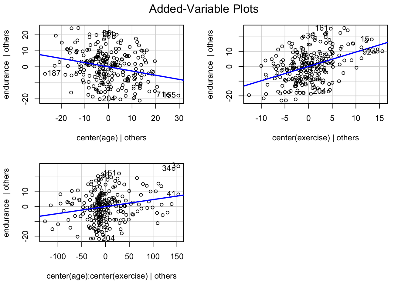
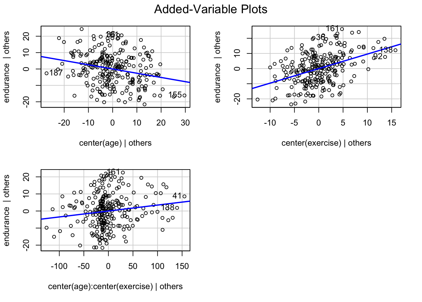
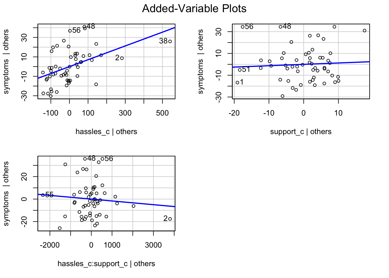
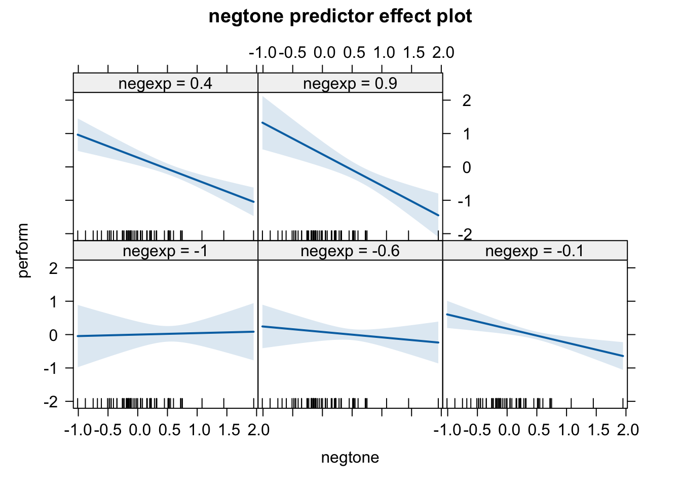
predictorEffects(mod_m, ~negtone) |>plot()
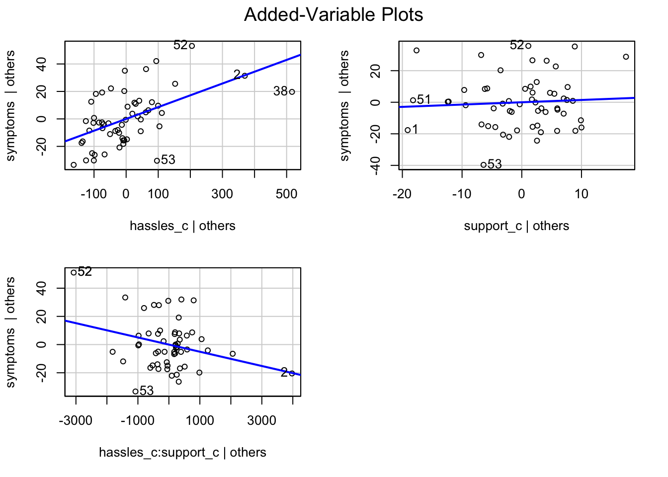
avPlots(mod_m)
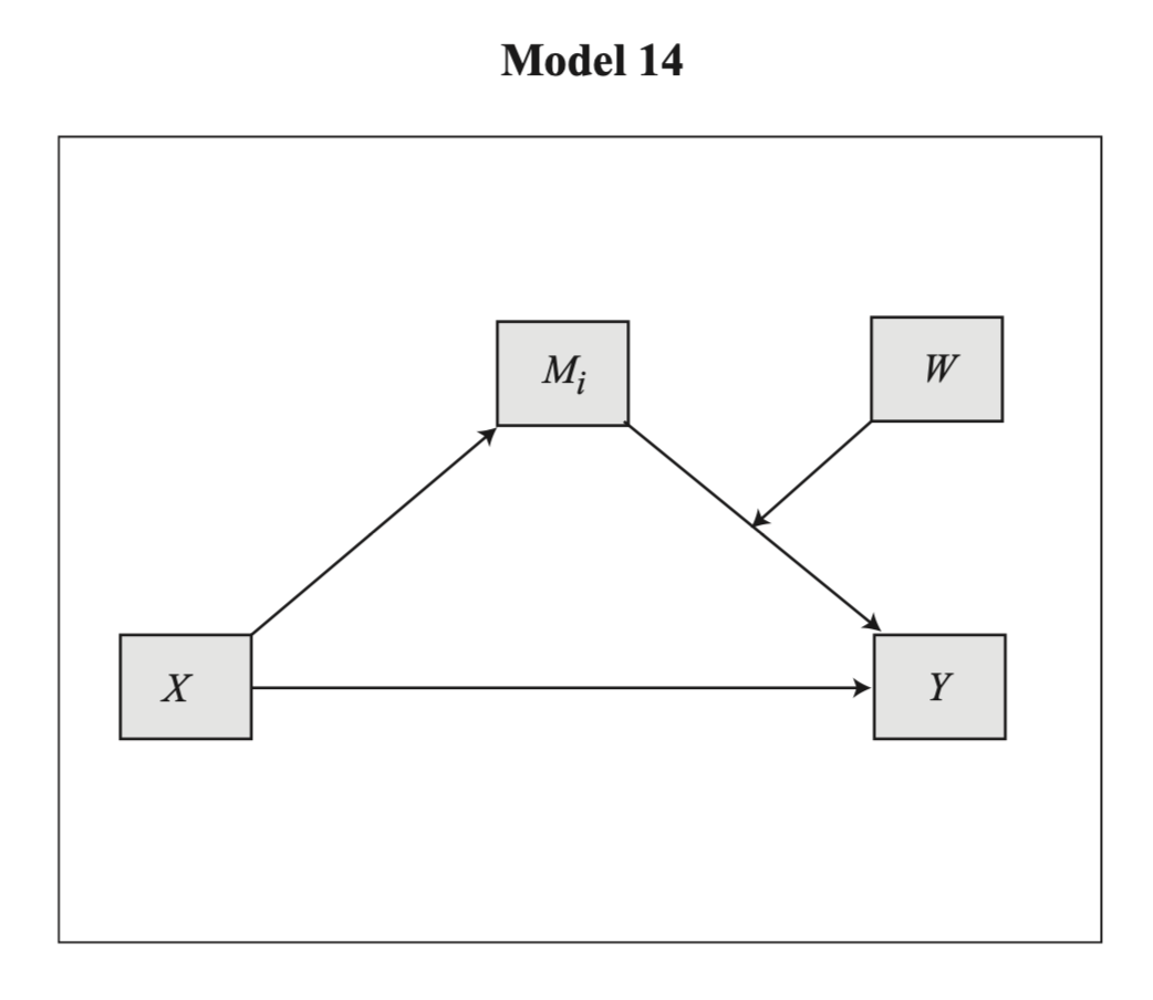
Hayes의 PROCESS를 매크로: Model 14
moments = 1: moderator의 세 값 (mean, mean +/- 1 SD)에 대한 조건적 효과를 계산
center = 1: centering
Index of moderated mediation: 조절변수가 1 변할 때, 간접효과의 변화가 얼마나 되는지를 나타내는 지수. 즉 간접효과가 얼마나 조절되는가?
process(data=teams, y="perform", m="negtone", w="negexp", x="dysfunc", jn=0, moments=1, center=1, model=14)# ********************* PROCESS for R Version 4.3.1 ********************* # Written by Andrew F. Hayes, Ph.D. www.afhayes.com # Documentation available in Hayes (2022). www.guilford.com/p/hayes3 # *********************************************************************** # Model : 14 # Y : perform# X : dysfunc# M : negtone# W : negexp # Sample size: 60# Random seed: 791081# *********************************************************************** # Outcome Variable: negtone# Model Summary: # R R-sq MSE F df1 df2 p# 0.4384 0.1922 0.2268 13.7999 1.0000 58.0000 0.0005# Model: # coeff se t p LLCI ULCI# constant -0.0215 0.0618 -0.3479 0.7292 -0.1451 0.1021# dysfunc 0.6198 0.1668 3.7148 0.0005 0.2858 0.9537# *********************************************************************** # Outcome Variable: perform# Model Summary: # R R-sq MSE F df1 df2 p# 0.5586 0.3120 0.2015 6.2350 4.0000 55.0000 0.0003# Model: # coeff se t p LLCI ULCI# constant -0.0321 0.0587 -0.5467 0.5868 -0.1496 0.0855# dysfunc 0.3661 0.1778 2.0585 0.0443 0.0097 0.7224# negtone -0.4314 0.1312 -3.2890 0.0018 -0.6943 -0.1686# negexp -0.0436 0.1134 -0.3841 0.7024 -0.2709 0.1838# Int_1 -0.5170 0.2409 -2.1458 0.0363 -0.9998 -0.0341# Product terms key:# Int_1 : negtone x negexp # Test(s) of highest order unconditional interaction(s):# R2-chng F df1 df2 p# M*W 0.0576 4.6043 1.0000 55.0000 0.0363# ----------# Focal predictor: negtone (M)# Moderator: negexp (W)# Conditional effects of the focal predictor at values of the moderator(s):# negexp effect se t p LLCI ULCI# -0.5437 -0.1504 0.2129 -0.7063 0.4830 -0.5770 0.2763# 0.0000 -0.4314 0.1312 -3.2890 0.0018 -0.6943 -0.1686# 0.5437 -0.7125 0.1530 -4.6565 0.0000 -1.0192 -0.4059# *********************************************************************** # Bootstrapping progress:# |>>>>>>>>>>>>>>>>>>>>>>>>>>>>>>>>>>>>>>>>>>>>>>>>>>>>>>>>>>>>>>| 100%# **************** DIRECT AND INDIRECT EFFECTS OF X ON Y ****************# Direct effect of X on Y:# effect se t p LLCI ULCI# 0.3661 0.1778 2.0585 0.0443 0.0097 0.7224# Conditional indirect effects of X on Y:# INDIRECT EFFECT:# dysfunc -> negtone -> perform# negexp Effect BootSE BootLLCI BootULCI# -0.5437 -0.0932 0.1537 -0.3751 0.2613# 0.0000 -0.2674 0.1193 -0.5282 -0.0591# 0.5437 -0.4416 0.1610 -0.7788 -0.1448# Index of moderated mediation:# Index BootSE BootLLCI BootULCI# negexp -0.3204 0.1887 -0.7753 -0.0491# ******************** ANALYSIS NOTES AND ERRORS ************************ # Level of confidence for all confidence intervals in output: 95# Number of bootstraps for percentile bootstrap confidence intervals: 5000# W values in conditional tables are the mean and +/- SD from the mean.# NOTE: The following variables were mean centered prior to analysis: # negexp negtone
Exercises
A. 다음 데이터는 the Octogenarian Twin Study of Aging에서 나타나는 패턴을 기반으로 생성한 데이터
includes 550 older adults age 80 to 97 years.
Cognition was assessed by the Information Test, a measure of general world knowledge (i.e., crystallized intelligence; range = 0 to 44)
demgroup 1: those who will not be diagnosed with dementia (none group = 1; 72.55%),
demgroup 2: those who will eventually be diagnosed with dementia later in the study (future group = 2; 19.82%)
demgroup 3: those who already have been diagnosed with dementia (current group = 3; 7.64%)