Base R

Author

Sungkyun Cho

Published

March 8, 2024

90년대에 통계 분석을 위해 개발된 R 언어와 대비하여, 좀 더 직관적이고 효율적인 데이터 분석을 위해 새로운 문법이 R내의 패키지 형태로 구현되었는데 이 새로운 생태계 안의 패키지들의 모임이 Tidyverse라는 이름하에 발전하고 있음: Tidyverse
이 패키지들은 design philosophy, grammar, data structures를 공유하며 유기적으로 작동됨.

기존 R의 문법과는 상당한 차이가 있어 단점도 지적되고 있고, 소위 base-R을 고수하는 사람들과 tidyverse를 기본으로 사용하는 사람들이 나뉘어 있다고 알려져 있음.

아마도 빠르게 발전하고 있는 tidyverse/tidymodel 생태계의 언어들이 기본으로 자리잡지 않을까 함.
본 강의에서는 주로 tidyverse의 언어로만 분석하고자 함.

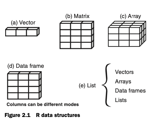
R의 데이터 구조와 변수 타입

주로 vector (벡터)와 data frame (데이터프레임)을 다룸

Source: R in Action by Rob Kabacoff

Data frame의 예

각 column이 하나의 variable (변수)를 구성하고, 한가지 타입의 데이터로 이루어짐
각 Row가 하나의 observation (관측치)을 구성함.
이러한 형태를 갖춘 데이터를 tidy라고도 부르며, 이를 벗어난 형태의 경우 가공이 필요함.
ex. “m23”: male이고 23세임을 나타내는 표기도 있음

library(tidyverse)

cps <- mosaicData::CPS85 # mosaicData package의 CPS85 데이터셋
head(cps) |> print() # print()는 생략할 것!

  wage educ race sex hispanic south married exper union age   sector
1  9.0   10    W   M       NH    NS Married    27   Not  43    const
2  5.5   12    W   M       NH    NS Married    20   Not  38    sales
3  3.8   12    W   F       NH    NS  Single     4   Not  22    sales
4 10.5   12    W   F       NH    NS Married    29   Not  47 clerical
5 15.0   12    W   M       NH    NS Married    40 Union  58    const
6  9.0   16    W   F       NH    NS Married    27   Not  49 clerical

cps <- as_tibble(cps) # tibble vs. data.frame
head(cps) |> print()

# A tibble: 6 × 11
   wage  educ race  sex   hispanic south married exper union   age sector  
  <dbl> <int> <fct> <fct> <fct>    <fct> <fct>   <int> <fct> <int> <fct>   
1   9      10 W     M     NH       NS    Married    27 Not      43 const   
2   5.5    12 W     M     NH       NS    Married    20 Not      38 sales   
3   3.8    12 W     F     NH       NS    Single      4 Not      22 sales   
4  10.5    12 W     F     NH       NS    Married    29 Not      47 clerical
5  15      12 W     M     NH       NS    Married    40 Union    58 const   
6   9      16 W     F     NH       NS    Married    27 Not      49 clerical

# Dataset의 설명
help(CPS85, package="mosaicData") # 또는
?mosaicData::CPS85

Vector

한 가지 타입으로만 구성: 숫자 (numeric), 문자 (character), 논리형 (logical), factor, etc

var <- c(1, 2, 5, 3, 6, -2, 4) # 변수에 assign: '=' 대신 '<-'
nm <- c("one", "two", "three")
tf <- c(TRUE, TRUE, TRUE, FALSE, TRUE, FALSE)

# 타입/클래스 확인
class(var)
## [1] "double"

class(nm)
## [1] "character"

class(tf)
## [1] "logical"

원소의 추출 및 대체

다음은 원소를 추출, 대체하는 R의 native한 방식임
수업에서는 뒤에서 다룰 tidyverse 문법을 주로 활용할 것임

Vector의 경우

var
## [1]  1  2  5  3  6 -2  4

var[3]
## [1] 5

var[c(1, 3, 5)]
## [1] 1 5 6

var[2:6] # ":"" slicing: c(2, 3, 4, 5, 6)
## [1]  2  5  3  6 -2

var[c(1, 3:5)] # 혼합
## [1] 1 5 3 6

var[-c(1, 3)] # "-"는 제외라는 의미
## [1]  2  3  6 -2  4

c(10, var, 100, 101) # 추가
##  [1]  10   1   2   5   3   6  -2   4 100 101

var[2] <- 55 # 대체
## var
## [1]  1 55  5  3  6 -2  4

var[c(2, 5)] <- c(200, 500) # 대체
## var
## [1]   1 200   5   3 500  -2   4

# numeric 벡터의 연산: recycling rule
1:5 * 2
## [1]  2  4  6  8 10

c(1, 3, 5) - 5
## [1] -4 -2  0

c(2, 4, 6) / 2
## [1] 1 2 3

c(1, 3) * c(2, 4)
## [1]  2 12

c(1, 3) - c(2, 4)
## [1] -1 -1

Factor

Vector로서 명목변수(카테고리)를 다룸

patientID <- c(1, 2, 1, 3)
diabetes <- c("Type1", "Type2", "Type1", "Type1")
status <- c("Poor", "Improved", "Excellent", "Poor")

# factor로 변환: 알파벳 순서로 levels의 순서가 정해짐
factor(patientID)
## [1] 1 2 1 3
## Levels: 1 2 3

factor(diabetes)
## [1] Type1 Type2 Type1 Type1
## Levels: Type1 Type2

factor(status, order = TRUE) # order를 표시
## [1] Poor      Improved  Excellent Poor     
## Levels: Excellent < Improved < Poor

# 구체적으로 표시하는 것을 추천: 지정한 성분 순서대로 levels의 순서가 정해짐
factor(status, levels = c("Poor", "Improved", "Excellent"),
                                         order = TRUE)
## [1] Poor      Improved  Excellent Poor     
## Levels: Poor < Improved < Excellent

# order가 없을시
factor(status, levels = c("Poor", "Improved", "Excellent"))
## [1] Poor      Improved  Excellent Poor     
## Levels: Poor Improved Excellent

# 대표적으로 성별을 코딩할 때: 숫자대신 레이블로 표시
sex <- c(1, 2, 1, 1, 1, 2, 2, 1)
factor(sex, levels = c(1, 2), labels = c("Male", "Female"))
## [1] Male   Female Male   Male   Male   Female Female Male  
## Levels: Male Female

sex_fct <- factor(sex, levels = c(1, 2), labels = c("Male", "Female"))

levels(sex) # 레벨 확인
## NULL
levels(sex_fct) # 레벨 확인
## [1] "Male"   "Female"

sex
## [1] 1 2 1 1 1 2 2 1
sex_fct
## [1] Male   Female Male   Male   Male   Female Female Male  
## Levels: Male Female

Data Frame

데이터 프레임의 구성

# 벡터들로부터 데이터 프레임 구성
patientID <- c(1, 2, 3, 4)
age <- c(25, 34, 28, 52)
diabetes <- c("Type1", "Type2", "Type1", "Type1")
status <- c("Poor", "Improved", "Excellent", "Poor")

patientdata <- data.frame(patientID, age, diabetes, status)

patientdata
##   patientID age diabetes    status
## 1         1  25    Type1      Poor
## 2         2  34    Type2  Improved
## 3         3  28    Type1 Excellent
## 4         4  52    Type1      Poor

midterm <- data.frame(english = c(90, 80, 60, 70),
                      math = c(50, 60, 100, 20),
                      class = c(1, 1, 2, 2))
midterm
##   english math class
## 1      90   50     1
## 2      80   60     1
## 3      60  100     2
## 4      70   20     2

원소의 추출 및 대체

# 원소의 추출
patientdata[1:2] # 변수의 열을 지정
##   patientID age
## 1         1  25
## 2         2  34
## 3         3  28
## 4         4  52

patientdata[c("diabetes", "status")] # 열 이름을 지정
##   diabetes    status
## 1    Type1      Poor
## 2    Type2  Improved
## 3    Type1 Excellent
## 4    Type1      Poor

patientdata[c(1, 3), c("age", "status")] # 행과 열을 모두 지정
##   age    status
## 1  25      Poor
## 3  28 Excellent

patientdata[c(1, 3), c(2, 4)]
##   age    status
## 1  25      Poor
## 3  28 Excellent

patientdata[, 1:2] # patientdata[1:2]과 동일, 빈칸은 모든 행을 의미
##   patientID age
## 1         1  25
## 2         2  34
## 3         3  28
## 4         4  52

patientdata[1:2, ] # 빈칸은 모든 열을 의미
##   patientID age diabetes   status
## 1         1  25    Type1     Poor
## 2         2  34    Type2 Improved

patientdata[-1] # 열 제외
##   age diabetes    status
## 1  25    Type1      Poor
## 2  34    Type2  Improved
## 3  28    Type1 Excellent
## 4  52    Type1      Poor

patientdata[-c(1, 3)] # 열 제외
##   age    status
## 1  25      Poor
## 2  34  Improved
## 3  28 Excellent
## 4  52      Poor

patientdata[-c(1:2), 2:4] # 행 제외 & 열 선택
##   age diabetes    status
## 3  28    Type1 Excellent
## 4  52    Type1      Poor


# 변수/열의 성분을 벡터로 추출: $ 또는 [[ ]]을 이용
patientdata$age # $를 이용
## [1] 25 34 28 52

class(patientdata$age) # numeric vector임을 확인
## [1] "numeric"

patientdata[["age"]] # patientdata$age과 동일, [[ ]] doule bracket을 이용해 벡터로 추출
## [1] 25 34 28 52

patientdata[[2]] # 열의 위치를 이용해도 동일한 추출
## [1] 25 34 28 52

patientdata["age"] # [ ] single bracket은 열을 선택하는 것으로 데이터 프레임으로 추출
##   age
## 1  25
## 2  34
## 3  28
## 4  52

patientdata[2] # 2번째 열을 추출; patientdata["age"]과 동일
##   age
## 1  25
## 2  34
## 3  28
## 4  52

데이터의 추가 및 대체

# 데이터 추가
patientdata$gender <- c(1, 1, 2, 2) 

patientdata
##   patientID age diabetes    status gender
## 1         1  25    Type1      Poor      1
## 2         2  34    Type2  Improved      1
## 3         3  28    Type1 Excellent      2
## 4         4  52    Type1      Poor      2

# 데이터 대체
patientdata[c(1,3), "age"] # 혼동: 원칙적으로 데이터프레임으로 추출되어야하나 벡터로 추출됨
## [1] 25 28

patientdata[c(1,3), "age"] <- c(88, 99)
patientdata
##   patientID age diabetes    status gender
## 1         1  88    Type1      Poor      1
## 2         2  34    Type2  Improved      1
## 3         3  99    Type1 Excellent      2
## 4         4  52    Type1      Poor      2

# 참고
row.names(patientdata) # 데이터 프레임의 행 이름
## [1] "1" "2" "3" "4"

row.names(patientdata) <- c("a", "b", "c", "d")
patientdata
##   patientID age diabetes    status gender
## a         1  88    Type1      Poor      1
## b         2  34    Type2  Improved      1
## c         3  99    Type1 Excellent      2
## d         4  52    Type1      Poor      2

Tibble

기존 data.frame의 단점을 보안한 tidyverse에서 기본이 되는 데이터 형식

Data frame vs. tibble

Printing의 차이

cps <- mosaicData::CPS85 # data.frame
cps
#   wage educ race sex hispanic south married exper union age   sector
# 1  9.0   10    W   M       NH    NS Married    27   Not  43    const
# 2  5.5   12    W   M       NH    NS Married    20   Not  38    sales
# 3  3.8   12    W   F       NH    NS  Single     4   Not  22    sales
# 4 10.5   12    W   F       NH    NS Married    29   Not  47 clerical
# 5 15.0   12    W   M       NH    NS Married    40 Union  58    const
# 6  9.0   16    W   F       NH    NS Married    27   Not  49 clerical
...

cps_tibble <- as_tibble(cps)
cps_tibble
# # A tibble: 534 × 11
#    wage  educ race  sex   hispanic south married exper union   age sector  
#   <dbl> <int> <fct> <fct> <fct>    <fct> <fct>   <int> <fct> <int> <fct>   
# 1   9      10 W     M     NH       NS    Married    27 Not      43 const   
# 2   5.5    12 W     M     NH       NS    Married    20 Not      38 sales   
# 3   3.8    12 W     F     NH       NS    Single      4 Not      22 sales   
# 4  10.5    12 W     F     NH       NS    Married    29 Not      47 clerical
# 5  15      12 W     M     NH       NS    Married    40 Union    58 const   
# 6   9      16 W     F     NH       NS    Married    27 Not      49 clerical
# # … with 528 more rows

그 외의 차이는 R for Data Science/10.3 Tibbles vs. data.frame을 참고